A brief introduction to networks

A network is quite a simple thing really, it’s a collection of nodes (sometimes called vertices), connected by paths (edges). A bit like this graph representing which characters know each other in the Batman universe (here the ‘nodes’ are characters and the ‘edges’ are the links between them):

Finding paths

One thing that can be important in analysing a network is finding a path through the network from one node to another. If the network was of say train stations (with the edges being connections between stations) then finding the path is analogous to planning a journey on the network.

But not all connections are made equally, sometimes there might be some restrictions on which paths can be taken, or some cost associated with taking a path. In the train example this might be indicative of journey time. Bringing this back to the network structure, each edge in the network is assigned a “weight” or “cost” that is indicative of how much energy/time is required to use that edge.

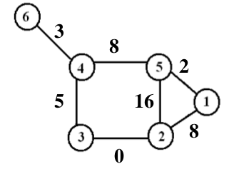
When we look for the “shortest path” between two nodes in a network, we use the weights on the edges that connect those two nodes. For example in the graph below, the shortest path from node 1 to node 6 is from node 1 to 5 to 4 to 6, with a total weight of 13.

This path can be found using Dijkstra’s algorithm (which is what my assignment was).

Dijkstra’s Algorithm

Dijkstra’s algorithm is really quite simple, but it can be a bit tricky to get your head around. I found this page from the University of Auckland really helpful in improving my understanding of it.

The algorithm uses the concept of a temporary and permanent label for each node. When the algorithm begins, all nodes have a temporary label representing their distance from the starting node. A typical value to initialise these labels to is infinity (or some other very large number). This represents the fact that the algorithm doesn’t know any of the distances yet. As the algorithm progresses, these labels will change (as we find paths to each node) and will be made permanent.

To begin with, the algorithm labels the starting point of the path with the permanent label 0 (as the start is “0 distance” from itself) and adds it to a set of nodes for which we have found the shortest path.

It then finds all the nodes that are connected to the starting node (its ‘neighbours’) and assigns them a temporary label equal to their distance from the start node. This distance is typically the weight on the edge between the neighbour and the start node. The neighbour with the smallest temporary label (i.e. the node that is closest to the start) has its label made permanent and we add it to the set of nodes that we have a path to.

This process is then repeated for the next closest node, but now we can use both a path that is direct from the starting node to a new node, or paths that go through the node we just labelled.

This is repeated until all nodes have a permanent label, which will give the shortest path from the start to any node in the network. Along the way it also keeps track of the “predecessors” of each node. The predecessors for a node are just the other nodes that lie on the shortest path from the starting point to that node. If this still isn’t clear, I’d recommend you check out this visual walk through provided by the University of Auckland.

def dijkstra(graph_dict, start, end):
    """
    This function implements Dijkstra's Shortest Path 
    
    It takes as its inputs:
        i. a graph represented by a "dictionary 
           of dictionaries" structure,
           i.e. {node: {neighbour: weight};
        ii. a starting node in that graph; and
        iii. an ending node for that graph
        
    The algorithm returns:
     i. the shortest path with 
     ii. its associated cost
    """
    # empty dictionary to hold distances
    distances = {} 
    # list of vertices in path to current vertex
    predecessors = {} 
    
    # get all the nodes that need to be assessed
    to_assess = graph_dict.keys() 
    # set all initial distances to infinity
    #  and no predecessor for any node
    for node in graph_dict:
        distances[node] = float('inf')
        predecessors[node] = None
    
    # set the initial collection of 
    # permanently labelled nodes to be empty
    sp_set = []
    # set the distance from the start node to be 0
    distances[start] = 0
    
    # as long as there are still nodes to assess:
    while len(sp_set) < len(to_assess):
        # chop out any nodes with a permanent label
        still_in = {node: distances[node]\
                    for node in [node for node in\
                    to_assess if node not in sp_set]}
        # find the closest node to the current node
        closest = min(still_in, key = distances.get)
        # and add it to the permanently labelled nodes
        sp_set.append(closest)
        
        # then for all the neighbours of 
        # the closest node (that was just added to
        # the permanent set)
        for node in graph_dict[closest]:
            # if a shorter path to that node can be found
            if distances[node] > distances[closest] +\
                       graph[closest][node]['weight']:
                # update the distance with 
                # that shorter distance
                distances[node] = distances[closest] +\
                       graph[closest][node]['weight']
                # set the predecessor for that node
                predecessors[node] = closest
                
    # once the loop is complete the final 
    # path needs to be calculated - this can
    # be done by backtracking through the predecessors
    path = [end]
    while start not in path:
        path.append(predecessors[path[-1]])
    
    # return the path in order start -> end, and it's cost
    return path[::-1], distances[end]

Summary

I had an awful lot of fun developing this algorithm. It was tricky at first, but once I’d got my head around what needed to be done, it was a blast. I should add that this probably isn’t the most efficient way to code this algorithm, and may not be the most “Pythonic” but it works for me and that (for now) is important.

I’d encourage anyone to have a go at implementing something similar themselves. It’s a tricky problem but you’ll get a real sense of achievement once you figure it out. Hopefully this post might help, too!

For those that are interested, you can see the full code, and grab the data for the example network I was working with from my Github repo.